7 Data Types

Variables can contain different types of data. These different data types will dictate both what types of analysis are appropriate and what chart types can best help us understand.

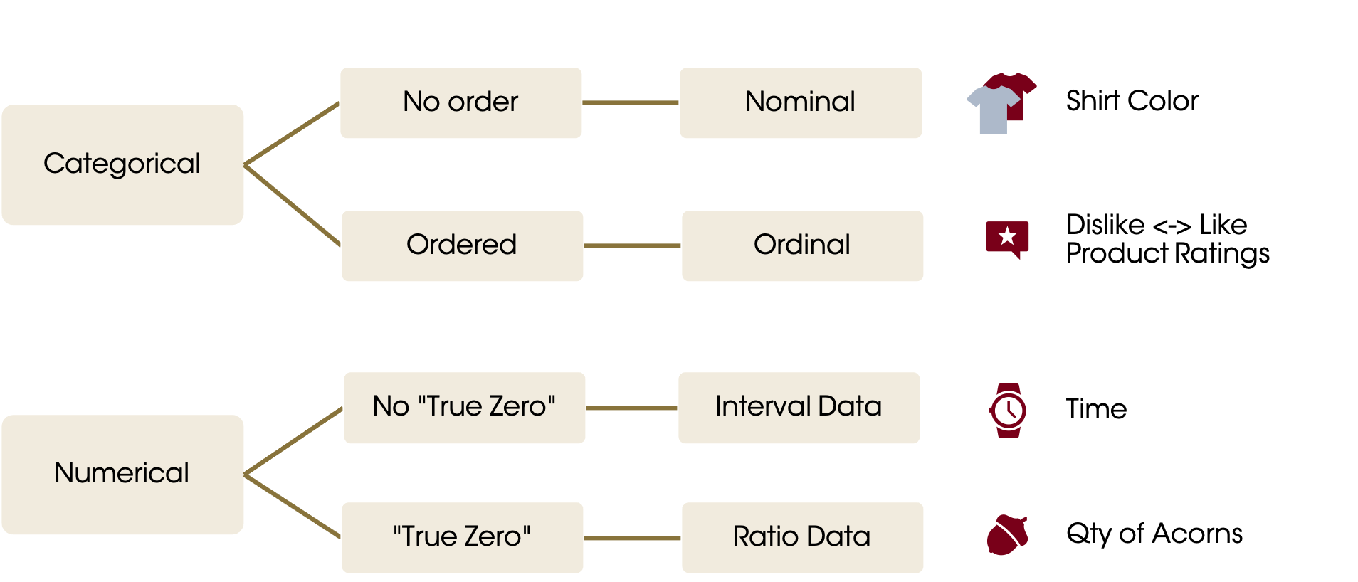
The chart below this shows the different types of data you may commonly encounter. This taxonomy is frequently used and was originally published by Stanley Stephens in Science in 1946. It is useful but not perfect.

7.1 Categorical Data

A variable that contains names or categories is referred to as categorical data. Categorical data is always discrete.

7.1.1 Nominal

Nominal data is called that because one definition of nominal is, “of or relating to a name.” The easiest example of nominal data is a people’s names! The key is that there is no inherent order to this data. Other examples include colors, music genres, movie titles, country names, etc.

We can count and categorize nominal data, but we can’t really do mathematical transformations on it. How do you “average” green and purple shirts? Brown?

7.1.2 Ordinal

Ordinal data has some order to it but is still categorical. Examples include: ratings from dissatisfied to satisfied, level of education (no high school diploma, high school, some college, associate’s degree, bachelor’s degree, graduate degree).

We can count and take the median, but we can’t “average” ordinal data. If we have a customer who is satisfied and one who is not satisfied, the “average” isn’t “somewhat satisfied.” There can also be big differences in the “distance” between categories. There’s a big difference between a high school diploma and a bachelor’s degree, but not as much difference between a bachelor’s degree and a master’s degree.

Note: You will often see ordinal data represented by numbers (e.g. 1-5 on a Likert scale). This data is often analyzed with statistical techniques such as taking the mean or using regression, but it’s not without controversy. For most things, it’s probably okay to transform well-designed survey data and analyze it using the mean. SS Stevens points out:

[F]or this ‘illegal’ statisticizing there can be invoked a kind of pragmatic sanction: In numerous instances it leads to fruitful results. While the outlawing of this procedure would probably serve no good purpose, it is proper to point out that means and standard deviations computed on an ordinal scale are in error to the extent that the successive intervals on the scale are unequal in size. When only the rank-order of data is known, we should proceed cautiously with our statistics, and especially with the conclusions we draw from them.

“On the Theory of Scales of Measurement.” Science. 1946. Vol 103, No 2684, pg 679

7.2 Numerical Data

7.2.1 Discrete vs. Continuous

Numerical data can be either continuous or discrete (sometimes you’ll see people argue that numerical data is all continuous; I disagree). Discrete data can only hold certain values. For example, the number of customers who shop in a store, or the number of students in a class. Continuous data can take any value in a range. For example, the time between two events.

We often approximate discrete events as continuous. For large samples, this can often be done without significant impacts. We also convert continuous variables, like income ($48,769), to discrete scales ($30-$50K).

7.2.2 Interval

Interval data has an inherent order and the difference between every unit on an interval scale must be the same. However, there is no true zero.

One example is time. The difference between any two intervals on the time scale (e.g. in minutes) is the same, but there’s no zero. Another example is credit scores, which range from 300-850. Finally, Chess player rankings range from 100-3000.

You cannot multiply or divide interval data (which means you can’t take percentages)! A 1500-ranked chess player isn’t “twice as good” as a 750-ranked player.

7.2.3 Ratio

Ratio data shares all the characteristics of interval data (ordered values on an equidistant scale) but has a true zero. Revenue, number of acorns, age, height of a building, etc are all ratio values.

7.3 Measurement Error and Data Limitations

Context and measurement matters. On the stock markets, trades can be made for fractions of a penny, but when you make a purchase in the store it will be rounded to the nearest penny when tax is calculated (Here’s the Minnesota state law specifying how that’s done).

Note any limitations of your instruments or of how the measurements are collected. You may have seen the HBO miniseries Chernobyl. Initial estimates were that the radiation levels were 3.6 Roentgen/hr; but the available dosimeters never anticipated such a disaster this was the highest dose they could measure. The true dose was 15,000 R/h. Anytime you see a “cliff” in your data, ask why.

7.4 Tricky Cases

It’s important to think through what the data type is because it can affect how you do your analysis. Consider day of the week. We can cross out ratio, because there is no zero-day. There IS a sort of order to them, but does the week start on Sunday or Monday? Does it matter if we just have one week’s worth of data (then we kind of DO have a zero, so maybe DoW represents time)?

The bottom line is that you need to think it through. Does your analysis make sense?

7.5 Calculations Possible by Data Type

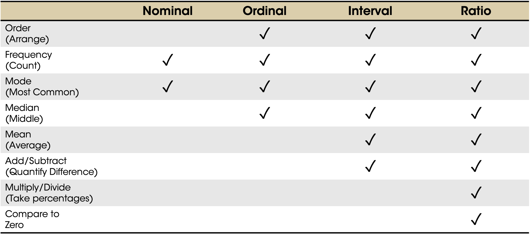
Different data types allow different types of calculations. Ask yourself, “Is this meaningful in the real world?” Note that your software won’t usually prevent you from attempting to do something “illegal” like average the values of a nominal variable.